Advertising adstock is the carry-over effect of some advertisement to a consumer over time. Finding the decay rate or half-life of advertising is a common question of interest to many advertisers to determine how effective advertising builds the awareness of their brand, and how that awareness decays over time.
Adstock is traditionally applied to advertisement via TV, and models are used to determine the best-fitting adstock rate of TV to Sales, or some sort of outcome (i.e. awareness). However in most cases, one would have other mediums such as Radio, Print, Digital, Social, etc.
I took the Nonlinear Least Squares approach to solving for the optimal adstock rate commonly applied to a single advertising medium, and augmented it to take in multiple variables.
My motivation for developing this multivariate approach is that modeling adstock rates for each advertisement medium independently may not be sufficient given that multiple mediums affect the outcome, and need to be accounted for collectively.
Method
Let 
 = adstock rate, and
  = error at time i. Then we can model Sales (or some outcome of advertising) as:

where

Now let’s say there are three advertising mediums that we want to compute adstock rates for. In this multivariate scenario, this model would look like this:

The goal is to find the optimal rates of all values, using Nonlinear Least Squares. The intercept that is computed from the model can also be interpreted as the Base, or the base level of sales or outcome if there were no advertising at all.
Example in R
For this example I generated a sample data with 3 ad variables (each representing some advertisement medium) with 104 obervations (representing roughly 2 years of weekly data). Then sales is generated from base + ad variables w/ ad stocking, with added random noise.
FYI: If you aren’t using pacman already, it is a great package management tool and I would highly recommend it (link to Github).
# generate sample data
pacman::p_load(minpack.lm)
set.seed(2222)

# adstock function
adstock <- function(x,rate=0){
  return(as.numeric(stats::filter(x=x,filter=rate,method="recursive")))
}

# generate base (intercept) + noise, and random values for ad1, ad2, and ad3
n_weeks = 104
base = 50
ad1 = sapply(rnorm(n_weeks, mean = 20, sd = 10), function(x) round(max(x, 0), 0))
ad2 = sapply(rnorm(n_weeks, mean = 20, sd = 10), function(x) round(max(x, 0), 0))
ad3 = sapply(rnorm(n_weeks, mean = 20, sd = 10), function(x) round(max(x, 0), 0))

# adstock rates
ad1_rate = .7
ad2_rate = .4
ad3_rate = .5

# generate sales data from the base + ad vairables w/ ad stocking, with random noise
sales = round(base + adstock(ad1, ad1_rate) + adstock(ad2, ad2_rate) + adstock(ad3, ad3_rate) + rnorm(n_weeks, sd = 5), 0)
I wrote a Multivariate Adstock Function in R, with special thanks to Angela Ju, whose code from this article I adopted and augmented. The equation from is implemented in the R function using the nls function to fit a nonlinear least squares with the adstock function.
This function can take a data.frame of any number of column(s) (or advertisement mediums), and will calculate the optimal adstock rate for each column in the input data.
(Note: for whatever reason, WordPress deletes portions of the code when publishing – if you want a working code to the function below, you can find it here).
#multivariate adstock function
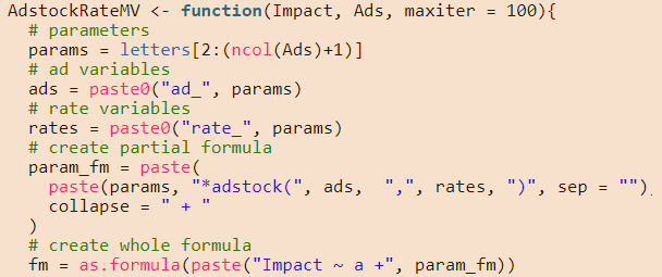
AdstockRateMV <- function(Impact, Ads, maxiter = 100){
# parameter names
params = letters[2:(ncol(Ads)+1)]
# ad variable names
ads = paste0("ad_", params)
# rate variable names
rates = paste0("rate_", params)
# create partial formula
param_fm = paste(
paste(params, "*adstock(", ads, ",", rates, ")", sep = ""),
collapse = " + "
)
# create whole formula
fm = as.formula(paste("Impact ~ a +", param_fm))
# starting values for nls
start = c(rep(1, length(params) + 1), rep(.1, length(rates)))
names(start) = c("a", params, rates)
# input data
Ads_df = Ads
names(Ads_df) = ads
Data = cbind(Impact, Ads_df)
# fit model
modFit rate_min) |
!all(summary(modFit)$coefficients[rates, 1] < rate_max)){
library(minpack.lm)
lower = c(rep(-Inf, length(params) + 1), rep(rate_min, length(rates)))
upper = c(rep(Inf, length(params) + 1), rep(rate_max, length(rates)))
modFit <- nlsLM(fm, data = Data, start = start,
lower = lower, upper = upper,
control = nls.lm.control(maxiter = maxiter))
}
# model coefficients
AdstockInt = round(summary(modFit)$coefficients[1, 1])
AdstockCoef = round(summary(modFit)$coefficients[params, 1], 2)
AdstockRate = round(summary(modFit)$coefficients[rates, 1], 2)
# print formula with coefficients
param_fm_coefs = paste(
paste(round(AdstockCoef, 2), " * adstock(", names(Ads), ", ", round(AdstockRate, 2), ")", sep = ""),
collapse = " + "
)
fm_coefs = as.formula(paste("Impact ~ ", AdstockInt, " +", param_fm_coefs))
# rename rates with original variable names
names(AdstockRate) = paste0("rate_", names(Ads))
# calculate percent error
mape = mean(abs((Impact-predict(modFit))/Impact) * 100)
# return outputs
return(list(fm = fm_coefs, base = AdstockInt, rates = AdstockRate, mape = mape))
}
The function takes in an Impact (a vector or single-column data frame of some advertising outcome), Ads (data frame of advertisement variables), and maxiter (maximum # of iterations for convergence), and returns the adstock model formula, base value, adstock rate for each ads considered, and the Mean average percent error (MAPE) between the predicted outcome and actual outcome.
First as a baseline, let’s fit a univariate model for adstock rates for each advertisement mediums.
# adstock for ad1
Impact = sales
(mod = AdstockRateMV(Impact, data.frame(ad1)))
## $fm
## Impact ~ 106 + 0.96 * adstock(ad1, 0.78)
##
##
## $base
## [1] 106
##
## $rates
## rate_ad1
##     0.78
##
## $mape
## [1] 6.9729
For Ad 1, the model estimates base as 106 and adstock rate as 0.78.
# adstock for ad2
(mod = AdstockRateMV(Impact, data.frame(ad2)))
## $fm
## Impact ~ 137 + 1.05 * adstock(ad2, 0.59)
##
##
## $base
## [1] 137
##
## $rates
## rate_ad2
##     0.59
##
## $mape
## [1] 8.064316
For Ad 2, the model estimates base as 137 and adstock rate as 0.59.
# adstock for ad3
(mod = AdstockRateMV(Impact, data.frame(ad3)))
## $fm
## Impact ~ 130 + 1.17 * adstock(ad3, 0.61)
##
##
## $base
## [1] 130
##
## $rates
## rate_ad3
##     0.61
##
## $mape
## [1] 7.768505
For Ad 3, the model estimates base as 130 and adstock rate as 0.61.
However, the original parameters used to simulate the data are base of 50 with rates of 0.7, 0.4, 0.5. To my previous point, modeling adstock for each medium independently may not be sufficient due to omitted-variable bias, and thus should be considered together.
Let us now compute the adstock rates for all three advertisement variables together in a multivariate model.
# multivariate adstock model
Ads = data.frame(ad1, ad2, ad3 )
(mod = AdstockRateMV(Impact, Ads))
## $fm
## Impact ~ 51 + 0.98 * adstock(ad1, 0.7) + 1.02 * adstock(ad2,
##     0.37) + 0.97 * adstock(ad3, 0.53)
##
##
## $base
## [1] 51
##
## $rates
## rate_ad1 rate_ad2 rate_ad3
##     0.70     0.37     0.53
##
## $mape
## [1] 2.160336
The model estimates base as 51 and adstock rates as 0.7, 0.37, 0.53. With a MAPE of 2.16%, and in comparison to base of 50 and rates of 0.7, 0.4, 0.5, this is a fairly accurate estimate.
Simulation
Now let’s do a simulation with n = 100 random samples taken from normal distributions.
# simulation
adstock_sim = function(){
  # generate base (intercept) + noise, and random values for ad1, ad2, and ad3
  base = 50
  ad1 = sapply(rnorm(n_weeks, mean = 20, sd = 10), function(x) round(max(x, 0), 0))
  ad2 = sapply(rnorm(n_weeks, mean = 20, sd = 10), function(x) round(max(x, 0), 0))
  ad3 = sapply(rnorm(n_weeks, mean = 20, sd = 10), function(x) round(max(x, 0), 0))
  # adstock rates
  ad1_rate = .7
  ad2_rate = .4
  ad3_rate = .5
  # generate sales data from the base + ad vairables w/ ad stocking, with random noise
  sales = round(base + adstock(ad1, ad1_rate) + adstock(ad2, ad2_rate) + adstock(ad3, ad3_rate) + rnorm(n_weeks, sd = 5), 0)
  # fit model
  Impact = sales
  Ads = data.frame(ad1, ad2, ad3 )
  mod = AdstockRateMV(Impact, Ads)
  return(c(base = mod[[2]], mod[[3]], mape = mod[[4]]))
}

# replicate 100 times
mod_rep = replicate(n = 100, adstock_sim())
rowMeans(mod_rep)
##      base  rate_ad1  rate_ad2  rate_ad3      mape
## 50.180000  0.699000  0.400900  0.492400  2.099492
With a simulation of 100 samples, the model estimates the average base as 50 and average rates as 0.7, 0.4, 0.5, with a mean MAPE of 2.1%.
The caveat here is that simulations can be built to produce any results as expected (and is certainly the case here), but in practice, I believe this multivariate approach to adstock modeling provides a better representation of adstock rates of different advertisment mediums, compared to a univariate approach.
If you liked this post, please feel free to leave a comment!

Hey Riki, awesome approach, really very cool. I did have a question about running this formula whil also adjusting for variables that are not advertising like number of locations, trend, seasonality, etc. Would you add another function that includes the other variables, then change the formula? Thanks!
LikeLike
Sorry I meant add another function argument
LikeLike
Hi Riki,
There is some non-syntactic code on line 24 of AdstockRateMV. Could you post a corrected version?
Thanks!
LikeLike
Hi Brian,
For some unknown reason, publishing to wordpress causes portions of the R code to disappear.
Please refer to the code in this markdown file on my github, the code there should work just fine:
https://github.com/rjsaito/Just-R-Things/blob/master/Statistics/mv_adstock.Rmd
LikeLike
Indeed it does. Thanks!
LikeLike
Hi Riki,
Can you also please show a sample function on how to get the optimal adstock rate?
Here in this example the adstock rates are fixed but according to my understanding, ideally we would like to get it from the model at which we get lest error.
LikeLike
Hello, I’m having a problem after running (mod(AdstockRateMV(x,y)). It gives the error code ‘Subscript out of bound”. I want to know if you have any insights into this. THanks
LikeLike
Hi. I am running a MMM model on multi-level data (DMA and time). I modified your adstock function to adstock by DMA groups. However, with this new adstock function I am not able to use the nls model for optimizing the adstock rate. I am sharing the code change below –
transfo %
group_by(DMANAME) %>%
mutate(adstock_col=transfo(Ad, 0.5))) %>% ungroup()
return(adstock_data$adstock_col)
}
I keep on getting the error – Singular gradient matrix with initial parameters.
LikeLike
How do you initialize the variable “start”? R throws an error as “element(12, 12) is zero so the inverse cannot be computed”.
LikeLike